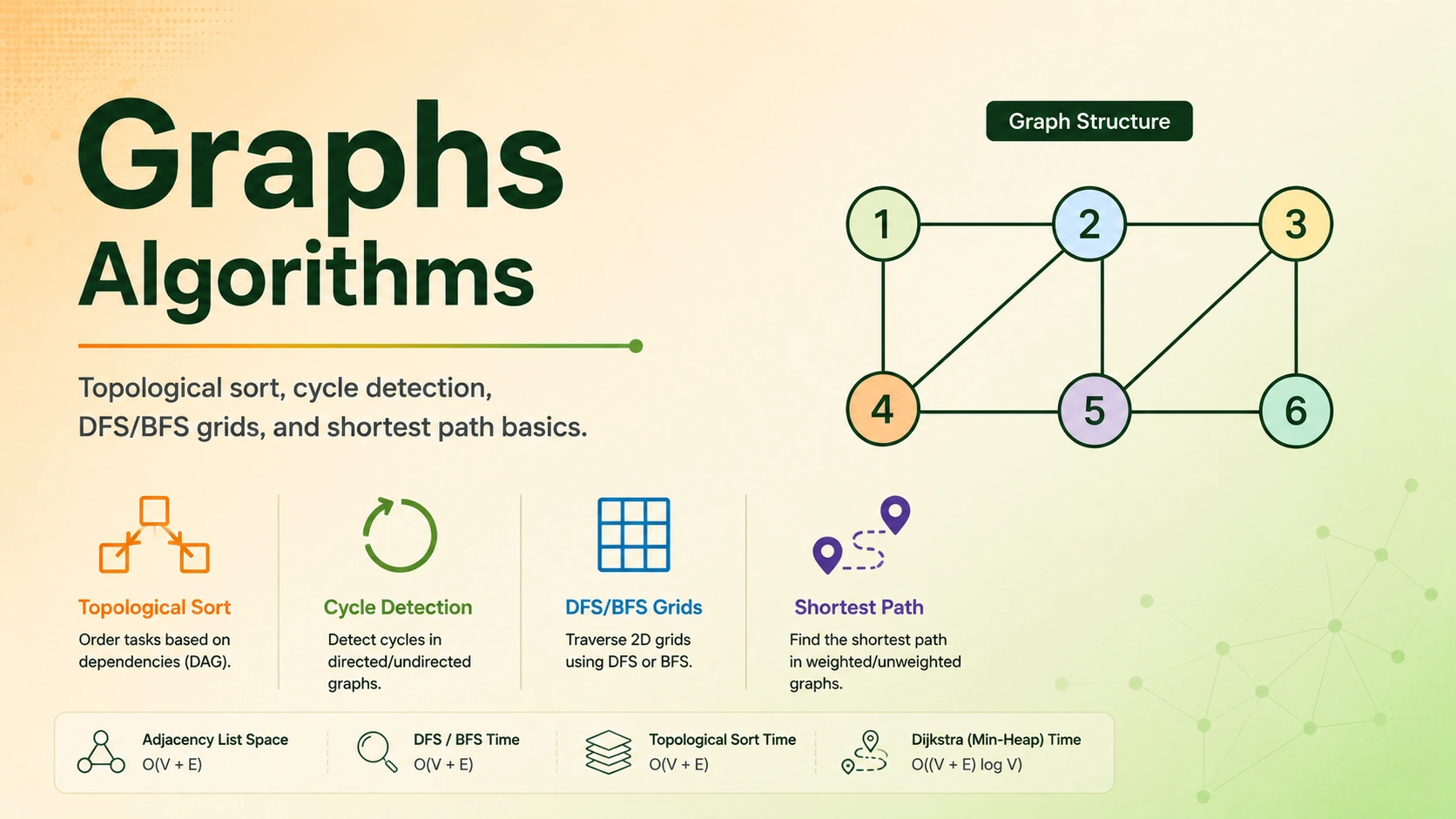
Introduction: The Social Network Map and the Flight Router
Imagine a social network like Facebook or LinkedIn. You have user profiles, and you have friendships connecting them. If Alice is friends with Bob, there is a connection. If Bob is friends with Charlie, there is another connection. But Alice might not be friends with Charlie directly.
This network of people and friendships is a real-world representation of a Graph.
In computer science, a Graph is a non-linear data structure consisting of two parts:
- Vertices (or Nodes): The entities in the graph (e.g., Alice, Bob, Charlie, cities, web pages).
- Edges: The relationships or connections between entities (e.g., friendships, flight paths, hyperlinks).
Graphs are versatile because they do not have a rigid hierarchical structure like Trees. Any node can connect to any other node, and there can be multiple loops or cycles in the paths.
Analogy: The Friend Map
Imagine a big map of your friends! Each friend is represented as a dot on a sheet of paper. If two friends know each other, you draw a line connecting their dots. In computer science, we call this a Graph!
- Vertices (or Nodes): The dots representing people, cities, or toys.
- Edges: The lines connecting the dots together.
- No rules!: Unlike a Tree, which grows in neat branches from the top, a Graph can connect any dot to any other dot. You can even have loops where you follow a path and end up right back at your starting spot!
Classifying Graphs
Directed vs. Undirected (Facebook Friends vs. Instagram Followers)
Analogy: Facebook vs Instagram
-
Facebook Friendship (Undirected): The friendship goes both ways! If Alice is friends with Bob, Bob is friends with Alice. The line has no arrows.
-
Instagram Follower (Directed): The follow has a direction! You follow a cool superhero account, but they might not follow you back. We draw this connection as a one-way arrow pointing from you to the superhero.
-
Undirected: The connection goes both ways. If Alice is friends with Bob, Bob is friends with Alice. The edge has no arrow.
-
Directed: The connection has a specific direction. If Alice follows Drake on Instagram, Drake does not automatically follow Alice. The edge is drawn as an arrow:
Alice -> Drake.
Weighted vs. Unweighted (Candy-toll Roads)
Analogy: Candy-toll Roads
-
Unweighted: Every connection is equal and free.
-
Weighted: Each path has a cost. Imagine walking between rooms in a board game, where some pathways require you to pay 5 candies to cross, but other paths only cost 1 candy. The candies are the Weights!
-
Unweighted: Every connection is equal.
-
Weighted: Connections have values or costs (weights). For example, in an airline routing system, an edge between New York and London might have a weight of
5,500(representing kilometers or flight costs).
Cyclic vs. Acyclic Graphs
- Cyclic: A graph containing at least one path that starts at a node and travels through edges to end up back at the same node.
- Acyclic: A graph with no cycles. A Directed Acyclic Graph is commonly known as a DAG and is key for scheduling algorithms.
Representing Graphs in Code
How do we represent nodes and edges in computer memory? We use three primary formats, each with distinct speed and memory trade-offs.
1. Adjacency Matrix
A 2D array of size V * V (where V is the number of vertices). If there is an edge between node i and node j, the cell matrix[i][j] is set to 1 (or the edge weight); otherwise, it is 0.
- Advantage: Instant
O(1)lookup to check if node A is connected to node B. - Disadvantage: Demands
O(V^2)memory. If you have 10,000 users but each user only has 5 friends, you waste huge amounts of memory storing millions of zeros.
2. Adjacency List
A mapping where each vertex is associated with a list or set of its neighbors. This is the most popular representation for interview coding because most graphs are sparse (nodes have relatively few edges).
- Advantage: Saves memory; requires only
O(V + E)space. - Disadvantage: Checking if node A connects to node B takes
O(degree of A)because you must search through A's list of neighbors.
Adjacency List Representation
(Nodes are represented as 0=A, 1=B, 2=C, 3=D for simplicity in the visualizer)
3. Edge List
A simple collection of pairs representing edges. E.g., edges = [[0, 1], [1, 2], [2, 3]].
- Use Case: Used as input in many problems (which you must first convert to an Adjacency List before traversing), and in Kruskal's Minimum Spanning Tree algorithm.
Complexity Matrix of Graph Formats
| Feature / Operation | Adjacency Matrix | Adjacency List | Edge List |
|---|---|---|---|
| Space Complexity | O(V^2) | O(V + E) | O(E) |
| Add Edge | O(1) | O(1) | O(1) |
| Check Edge Connection | O(1) | O(deg(V)) | O(E) |
| Find All Neighbors | O(V) | O(deg(V)) | O(E) |
Core Graph Traversals: BFS vs. DFS
To traverse a graph, we must visit its vertices. Since graphs can have loops, we must keep track of nodes we have already visited to avoid falling into infinite loops. We do this using a Visited Set.
Analogy: Secret Hideouts in the Playground
Imagine you are exploring a web of secret hideouts in a giant playground! How do you visit every single hideout without getting lost in loops? You bring a bucket of green slime to mark each hideout you visit (we call this a Visited Set so we don't walk in circles forever!).
There are two main strategies to explore this web of hideouts: Breadth-First Search (BFS) and Depth-First Search (DFS).
1. Breadth-First Search (BFS): The Ripple in a Pond
Visualize Breadth-First Search exploring a graph layer-by-layer starting from a source node.Graph BFS
Imagine dropping a pebble in a puddle of water—it creates ripples that spread outwards in growing circles. BFS works exactly like this!
How it works step-by-step:
- You start at your house (the starting node).
- First, you visit all of your direct next-door neighbors (Level 1).
- Next, you visit all of their next-door neighbors (Level 2).
- You keep spreading outwards layer-by-layer.
Why we use it: Because BFS searches everywhere 1 step away, then 2 steps away, and so on, it is the perfect way to find the absolute shortest path to any destination!
How we code it: We use a Queue (a First-In-First-Out line, like waiting for a water slide). You get in line, visit a hideout, mark it as visited, and put all its unvisited neighbors at the back of the line!
2. Depth-First Search (DFS): The Deep Maze Explorer
Visualize Depth-First Search as it explores a graph by going deep along each branch before backtracking.Graph DFS
Imagine exploring a deep, dark maze. You don't spread out; you pick a direction and commit to it!
How it works step-by-step:
- You pick a path and walk as far as you can possibly go until you hit a dead end.
- Once you hit a wall, you walk back (this is called backtracking) to the last intersection.
- From that intersection, you try the next unexplored path!
- You explore deep before you explore wide.
Why we use it: It is perfect for checking if a path exists between two places, solving mazes, or finding cycles (checking if you walked in a circle).
How we code it: We use Recursion (a function calling itself) or a Stack (a Last-In-First-Out tower, like a stack of pancakes). You always explore the most recently discovered path first.
Side-by-Side Comparison
| Metric | BFS (Breadth-First Search) | DFS (Depth-First Search) |
|---|---|---|
| Exploration Style | Wide and shallow (Layer-by-layer) | Deep and narrow (Plunges to the bottom) |
| Data Structure | Queue (FIFO) | Stack / Recursion (LIFO) |
| Memory Usage | O(width) (stores all nodes of a level) | O(depth) (stores the recursion path) |
| Shortest Path | Guaranteed to find the shortest path (unweighted) | Not guaranteed to find the shortest path |
| Best For | Finding nearest neighbors, shortest path | Topological sort, cycle detection, maze solving |
Key Algorithmic Patterns
Pattern 1: Grid BFS/DFS (The Island Problem)
Visualize DFS/BFS flood-fill on a 2D grid to count distinct connected land masses surrounded by water.Number of Islands
- The Strategy:
- Iterate through every cell in the grid.
- If you find land (
'1'), trigger a DFS or BFS to visit and mark all connected land cells as water ('0') or visited. - Increment your island count.
Grid DFS Traversal Template
Pattern 2: Topological Sort (Kahn's Algorithm)
See how topological ordering resolves dependencies in a Directed Acyclic Graph (DAG) using DFS or Kahn's algorithm.Topological Sort
U -> V, vertex U comes before V in the ordering.
- Real-world Example: Course scheduling. If Course A is a prerequisite for Course B, you must take A before B.
- Kahn's Algorithm:
- Calculate the in-degree (number of incoming edges) for every vertex.
- Add all vertices with an in-degree of 0 (no prerequisites) to a Queue.
- While the queue is not empty:
- Pop a vertex from the queue, add it to our sorted output.
- Decrement the in-degree of all its neighbors.
- If a neighbor's in-degree drops to 0, push it onto the queue.
- If the sorted output does not contain all vertices, a cycle exists, and topological sort is impossible.
Kahn's Algorithm Implementation
Pattern 3: Shortest Path on Weighted Graphs (Dijkstra's Algorithm)
Visualize finding the shortest paths from a single source vertex to all other vertices in a weighted graph.Dijkstra's Algorithm
To find the shortest distance from a starting node to all other nodes in a weighted graph with non-negative weights, we use Dijkstra's Algorithm.
It uses a Min-Heap (Priority Queue) to always explore the next node that has the absolute shortest path distance from the start.
Dijkstra's Template
Pattern 4: Disjoint Set Union (DSU / Union-Find)
The Disjoint Set Union (Union-Find) data structure tracks elements split into non-overlapping subsets. It is useful for:
- Cycle detection in undirected graphs.
- Kruskal's algorithm (Minimum Spanning Tree).
- Finding connected components in dynamic graphs.
DSU implements two main operations:
- Find: Determine which subset an element belongs to (returns the representative or parent of the set).
- Union: Join two subsets into a single subset.
DSU Optimization: Path Compression & Union by Rank
Without optimization, DSU find operations can degrade to O(n) if elements form a long linear chain. We use two tricks:
- Path Compression: During a
findcall, we update the parent pointer of every node visited to point directly to the root. This flattens the tree. - Union by Rank: Always attach the smaller tree (lower rank) under the root of the larger tree (higher rank) to keep the depth balanced.
Union-Find Implementation
Complete Graph Traversals in 4 Languages
Let's write standard BFS on an adjacency list in Python, Java, C++, and TypeScript.
Step-by-Step Kahn's Course Schedule Trace
Suppose we have numCourses = 3 and prerequisites = [[1, 0], [2, 1]].
This means:
- Course 0 must be taken before Course 1 (
0 -> 1). - Course 1 must be taken before Course 2 (
1 -> 2).
1. Initial State
- In-degrees:
{0: 0, 1: 1, 2: 1} - Adjacency list:
{0: [1], 1: [2], 2: []} - Queue:
[0](since in-degree of 0 is 0).
2. Trace Table
| Step | Node Popped | Neighbors checked | In-degree changes | Nodes pushed to Queue | Visited Count |
|---|---|---|---|---|---|
| 1 | 0 | 1 | In-degree of 1 drops to 0 | [1] | 1 |
| 2 | 1 | 2 | In-degree of 2 drops to 0 | [2] | 2 |
| 3 | 2 | None | - | None | 3 |
- Termination: Queue is empty. Visited Count is 3, which equals numCourses. We can complete all courses!
Common Interview Pitfalls and Debugging Strategies
-
Cycle Infinitum:
- Symptom: Your traversal runs forever and hits a stack overflow or timeout.
- Cause: You forgot to register visited nodes in your Visited Set, causing you to revisit the same loop repeatedly.
- Fix: Always mark the starting node as visited immediately before pushing it to a queue or executing the recursion step.
-
Index Out of Bounds in Grids:
- Symptom:
IndexOutOfBoundsExceptionorundefinedreads during grid traversal. - Cause: You forgot to check boundaries before accessing
grid[r][c]. - Fix: Validate borders first:
if r < 0 or r >= rows or c < 0 or c >= cols: return.
- Symptom:
-
Directed Cycle Detection DFS (Three-State Coloring):
- Symptom: Traditional visited sets fail to detect cycles in directed graphs.
- Cause: A node might be visited from two independent paths without there being a cycle.
- Fix: Use a three-state marker array (0 = unvisited, 1 = visiting/on stack, 2 = fully processed). A cycle is detected only if you encounter a neighbor in the 'visiting' state.
Practice Problems & Website Verifications
Verify your graph traversals and scheduling algorithms on our platform:
- Number of Islands — Run 4-directional DFS to count components.
- Clone Graph — Traverse using a Hash Map to clone deep nodes.
- Course Schedule — Implement Kahn's Topological Sort.
Interactive Visualizations
Engage with these concepts dynamically. Click on any card below to launch the interactive simulator and step through the algorithm execution.
Graph DFS
Visualize Depth-First Search as it explores a graph by going deep along each branch before backtracking.
Graph BFS
Visualize Breadth-First Search exploring a graph layer-by-layer starting from a source node.
Topological Sort
See how topological ordering resolves dependencies in a Directed Acyclic Graph (DAG) using DFS or Kahn's algorithm.
Dijkstra's Algorithm
Visualize finding the shortest paths from a single source vertex to all other vertices in a weighted graph.
Number of Islands
Visualize DFS/BFS flood-fill on a 2D grid to count distinct connected land masses surrounded by water.